Goals:
Walk through a options navigating within a Jupyter Notebook session
Demonstrate options and features available in Jupyter Notebooks
...
| Table of Contents | ||||||||
|---|---|---|---|---|---|---|---|---|
|
Click to start
OnDemand interactive applications can be launched from OnDemand with graphics, similar to a remote desktop that only launches the application.
After logging into OnDemand on your favorite ARCC HPC resource, you can request a Jupyter Session by clicking on the app from the main Dashboard:
...
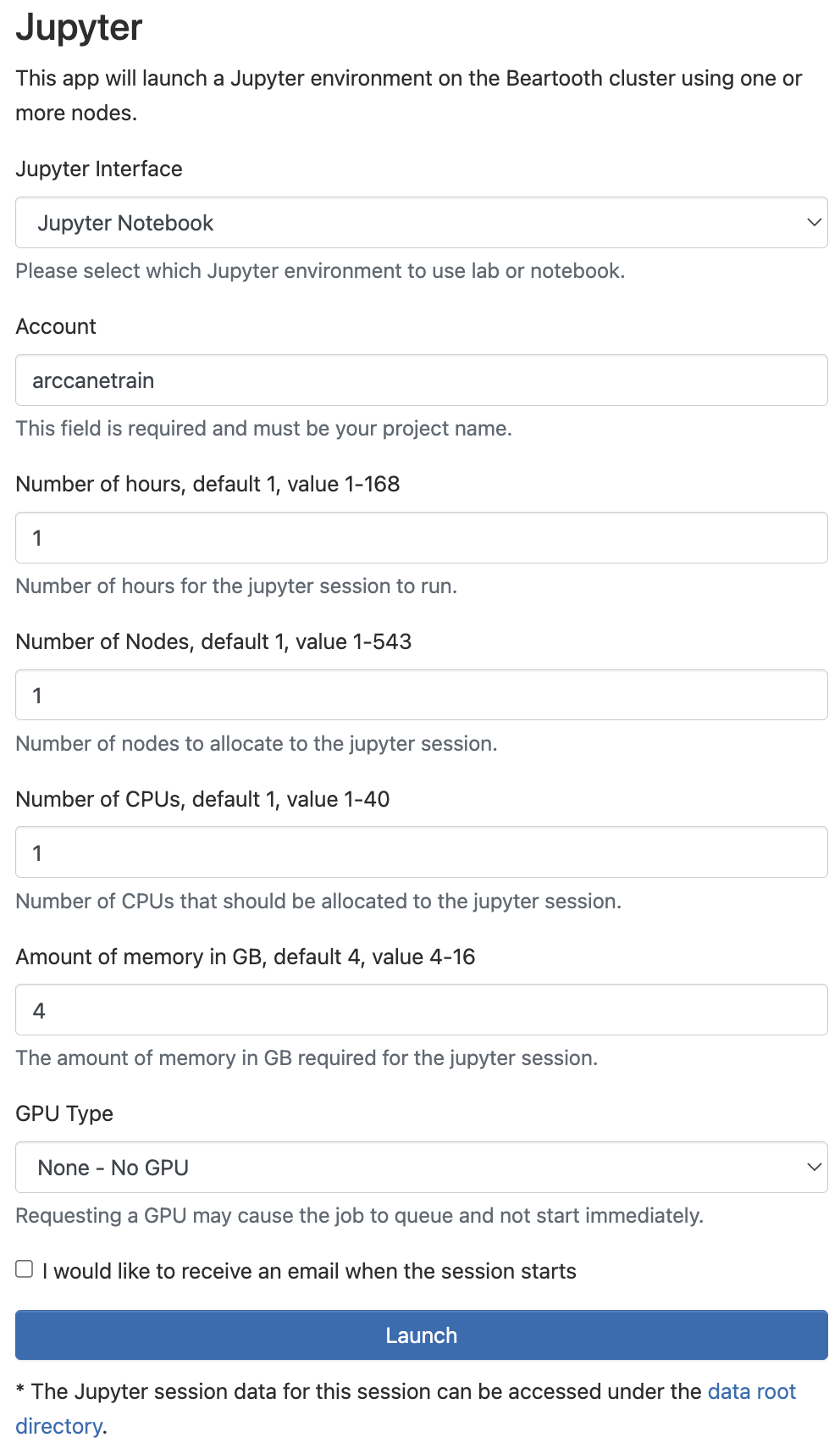
Fill out the Jupyter Session Request Form
After clicking the jupyter app, you are taken to a web form to tailor and specify the Jupyter environment you’d like to run in your session
Jupyter Interface: Select from Jupyter Notebook or Jupyter Lab
Account: The associated investment account or project you’re using to run the session
Number of hours: How long you plan to use the notebook
Number of Nodes: how many nodes you want allocated to perform work while using this notebook.
Number of CPUs: how many cores you will need access to perform your work while using this notebook.
Amount of Memory: Memory in GB required to run throughout the course of this Jupyer session
GPU Type: Which GPU hardware you’d like to perform your work in the Jupyter Notebook or Lab on
...
Your interactive sessions
...
When you click launch, you’re redirected to a page showing a list of your most recent interactive sessions.
The Slurm scheduler assigns a compute node with a specified number of cores, memory, hardware and timeframes as requested from the input you provided in your webform.
When your session is ready for use, the heading will turn green.
Completed sessions are denoted with gray headings
Pending sessions are denoted with blue headings
...
.
...
Connect to your session
...
To open Jupyter, click on the connect button within the active session
...
You will be directed to a Jupyter notebook or lab environment to start using Jupyter!
...
Starting Jupyter from OnDemand
|
...
Initial Screen Navigation and Options
Upon connecting, you are presented the jupyter dashboard which serves as your home page for jupyter notebook. The Jupyter Notebook screen is rather simple with 3 tabs:
|  |
|---|
...
What are Kernels?
A Jupyter kernel is the computational engine behind the code execution in Jupyter notebooks.
Most users think of this as the “compiler” or programming language used when running code cells.
The Kernel empowers you to execute code in different programming languages like Python, R, or Julia or other languages and instantly view the outcomes within the notebook interface.
Once you open a new notebook, you may be prompted to select a kernel
|  |
Default Kernels on ARCC HPC Resources currently include:
HPC-wide kernels are titled by packages installed and available when launched Users can also create user-defined kernels from conda environments (Covered in a subsequent module. See: Launching Jupyter Kernels from Conda Environments) |  |
...
Open a New Blank Notebook
From the Right side of the File Management Tab: New->Notebook-> Select from a list of kernels. Choose This should open a new browser tab/window with a blank Jupyter notebook named: If we go back to our previous Jupyter tab/window containing the file browser from which we launched our notebook, this new file shows up in the list, and has a green icon to it’s left, meaning it is currently running:  |  |
...
New Notebook - New Options
When a notebook is open a new browser tab is created showing the notebook user interface (UI).
This allows for interactive editing and running of the notebook document.
|  |
...
Menu Bar with Dropdowns
Note: Jupyter extensions can create new top-level menus in the menu bar. |  |
Right of the menu bar, the current kernel is listed |  |
...
Toolbar Actions
|
|


...
Notebook Cell Types
We can use the cell type option in the toolbar to set cell type in the notebook body:
|  |
...
Code
|  |
|---|
...
Markdown
|  |
|---|
...
Raw NBConvert
|  |
...
Where are we?
Previously, we said the file management tab shows the filesystem accessible to the user, rooted by the directory from which the notebook was launched. In the file management tab we can see root directory, and within it, the doc and ondemand folders. We could just assume the file manager is showing our home directory. But how would we find out for certain? |  |
...
Running with a Python kernel, we can use our jupyter notebook to get this information from the system:
Note: New input cells are code cell types by defaultWith the information from our output cell, we can conclude that OnDemand launches Jupyter from your $HOME | 
|
...
Another way:
Running with a Python kernel, we can use our jupyter notebook to get this information from the system with ! implementation to run a command from the shell of the underlying system:
Note: New input cells are code cell types by defaultWith the information from our output cell, we can conclude that OnDemand launches Jupyter from your $HOME | 
|
...
How to get to directories outside of $HOME?
If we select the default Python 3 (ipykernel), we are presented with the file explorer showing our home directory as it’s rooted location. This means we can’t go up any further in system’s directory structure.
|  | |||||
|
|

...
Or, lets get clever:
Alternatively, we can simplify things by create a symbolic link from within our notebook using ! functionality (if we’re running an ipython kernel): |  |
...
Can we get outside of home now?
We can see new links to our external directories: |  |
And now we can get to them: |  |
...
Getting information about packages?
What’s Installed - How to find out:
In our notebook, we can see which modules are available by opening a new cell with the + button. In our cell box, set as “code” use the python Hitting tab after |
 |
...
What’s Installed - Can we get a list in Python?
Yes. By running |
 |
...
What’s installed and how to use it: Python - help()
Generally,
help ('modules <module_name>')will give us information on how to use the specific python library we’re importing as long as that library is installed.Similar in functionality to the
--helpandmancommands for shell.
...
What’s Installed - Can we get a list in R?
...
What’s Installed - Query a specific package in R?
...
What’s Installed and how to use it: In R - help()
...
We’ve confirmed the package we need is unavailable:
Our output results in an error: |
 |
|
...
Option 1: Load a different kernel
Depending on the HPC’s native environment, you may have other kernels available. |  |
Or not ---> MedBow currently has a minimal number of global kernels (purposefully). |  |
...
If this were an option, we’d see it in our dropdown list of kernels and could select a different one:
|
 |
...
The new kernel is loaded as shown in the top right of our notebook.
|  |
|  |
...
No available kernels have all the software I need - Now what?
Partially covered in python and conda materials, but short answer:
Best practice - Do NOT install the software directly from your jupyter kernel
...
...
Doing so can and frequently does eventually result in:
...
...
Next Steps
Previous | Workshop Home | Next |